There are many examples provided in the \example directory. Some examples are described below, but there are more examples in the DyRoBeS\Example directory. You are encouraged to go through all the examples.
Example 1: 2-Axial Groove Bearing
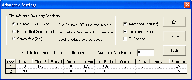
File: Brg_2-Axial_Groove_Coor1.LDI – Lund Coordinate System
File: Brg_2-Axial_Groove_Coor2.LDI – Standard Coordinate System
File: Brg_2-Axial_Groove_Coor2.LDI – Metric Units
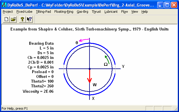
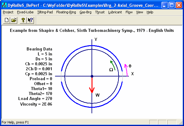
This example is taken from Shapiro & Colsher, Sixth Turbomachinery Symp., 1979. It is a 2-axial groove bearing as shown below:

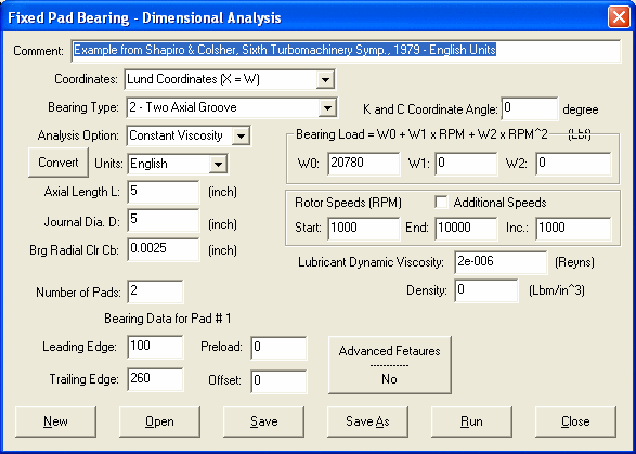
For comparison purposes with previous publications, the X-axis is aligned with the load vector (Lund coordinate system) and constant viscosity is used in File: Brg_2-Axial_Groove_Coor1.LDI. Since two lobes are identical, no discontinuity in the bearing clearance, and the turbulence effect is neglected, therefore, Advanced Feature is turned off (unchecked). The bearing parameters are listed below for reference.
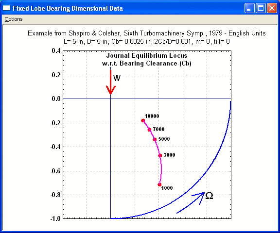
The journal equilibrium locus is shown below.
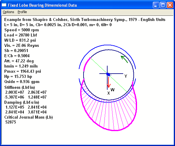
The bearing performance at 5000 rpm is shown and the results are in agreement with previous publications.
By selecting the Standard Coordinate System, an additional input for load vector, 270o in this case, is needed as demonstrated in File: Brg_2-Axial_Groove_Coor2.LDI. Again, for comparison purposes, the bearing coefficients are oriented such that the x-axis is collinear with the load vector as shown in the input. The results are identical with previous discussion.
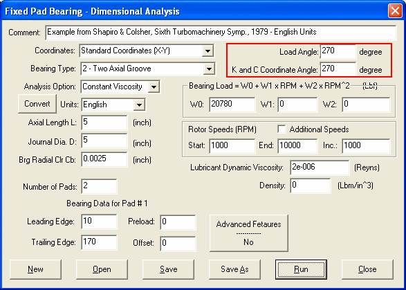
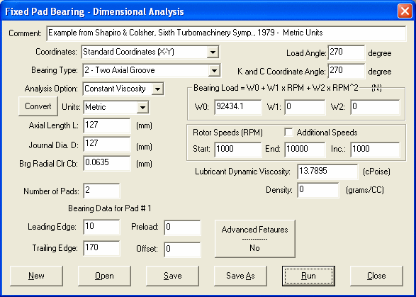
The input parameters can also be in metric units as demonstrated in File: Brg_2-Axial_Groove_Coor2_mm.LDI and shown below.
Example 2: 3 Lobe Bearing – Laminar and Turbulent Flow
A 3 lobe bearing as shown below is used in a high-speed application. The load vector is directed in the middle of the lobe.
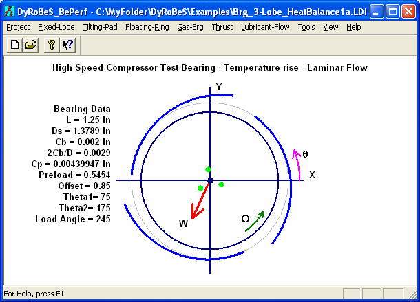
The bearing clearance for each lobe is continuous along the circumferential direction, although it is not a constant due to the preload. Each lobe is identical. Two cases are studied, one is laminar flow and second one is turbulent flow. With laminar flow assumption, the input parameters are shown below with Advanced Feature OFF:
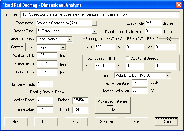
The bearing performance at 48,000 rpm is shown below. With 120o F oil inlet temperature, the operating and maximum bearing temperatures are 154o and 191o F with laminar flow assumption.
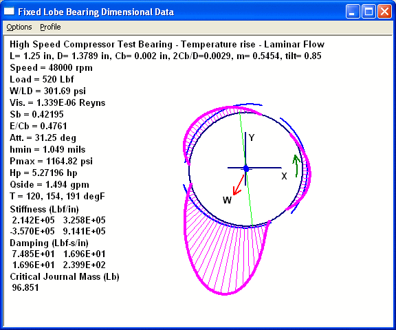
With the Advanced Feature OFF, the laminar flow is assumed. Also, without Advanced Feature, each finite element node has one (1) degree-of-freedom, i.e., pressure is the only unknown at each finite element node. With Advanced Feature ON, the turbulent effect can be included or neglected. Also, with Advanced Feature ON, each finite element node has three (3) degrees-of-freedom, i.e., pressure and pressure gradients in axial and circumferential directions are the unknowns at each finite element node. With turbulent flow assumption, the input parameters are shown below with Advanced Feature ON:
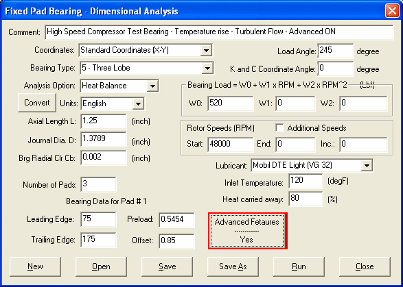
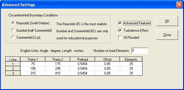
The bearing performance at 48,000 rpm is shown below with turbulence effect CHECKED, With 120o F oil inlet temperature, the operating and maximum bearing temperatures are 158o and 195o F.
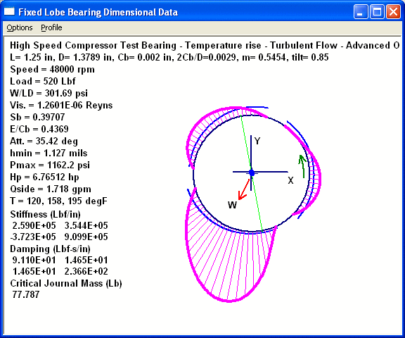
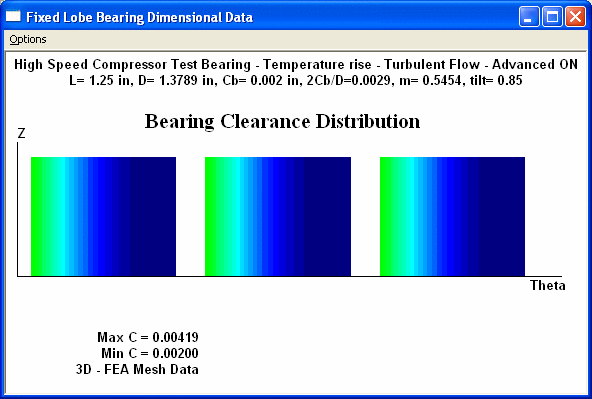
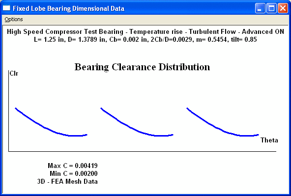
With Advanced Feature ON, the bearing clearance can be easily checked as shown below in top view and side view.
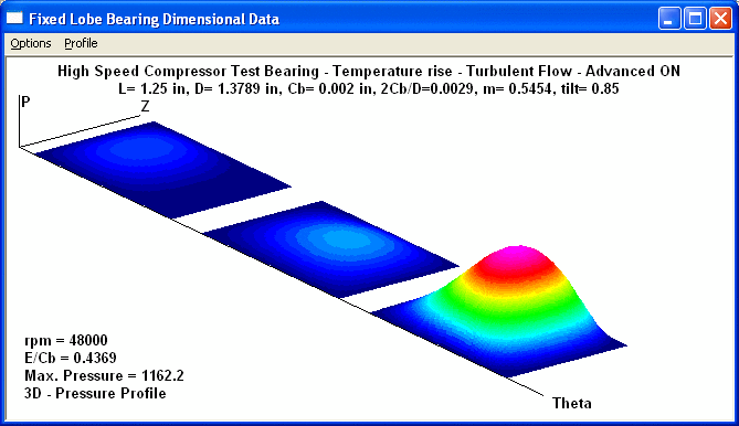
A 3 dimensional pressure profile can also be viewed.
Example 3: Pressure Dam Bearings
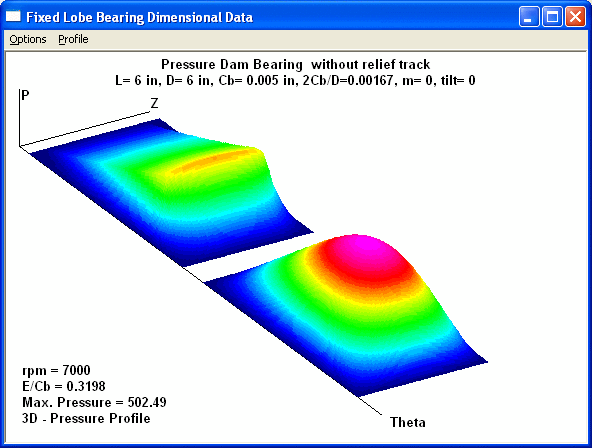
A conventional pressure dam bearing is demonstrated in this example. A pressure dam (pocket) with a constant depth is in the top lobe, and a central relief track with much larger depth is in the lower lobe where the load vector is located. The bearing geometry with exaggerated clearance and bearing clearance distribution are shown below:
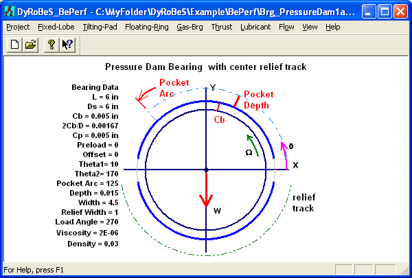
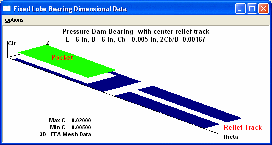
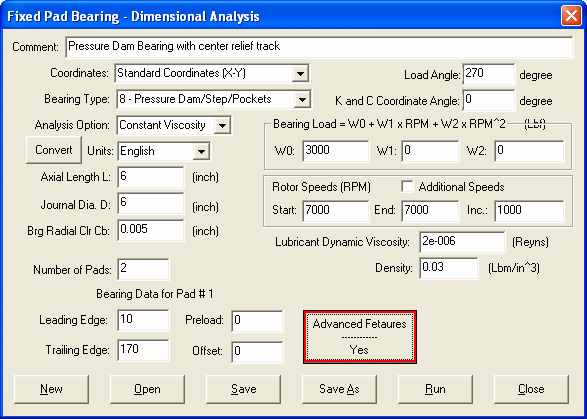
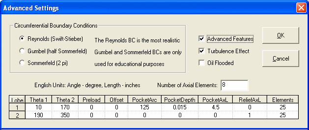
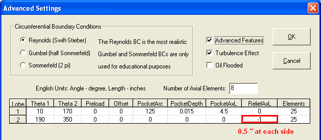
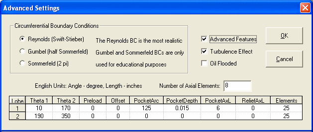
The pressure dam bearing has discontinuity in the bearing clearance. Therefore, the Advanced Feature must be turned ON. Additional data for the pocket and relief track are entered in the Advanced Feature dialog box. The computer program allows for the pocket and relief track in a preloaded lobe, although typically they are in a plain lobe without any preload. Note that the pocket axial length (PocketAxL) must be smaller than the bearing axial length in order to have a pocket with side dams. If PocketAxL equals to the bearing axial length, then it becomes a step bearing without side lands which is acceptable in this program. The pocket and relief track cannot co-exist.
The bearing performance and pressure distribution are shown below.
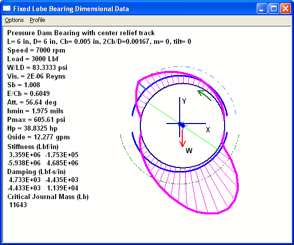
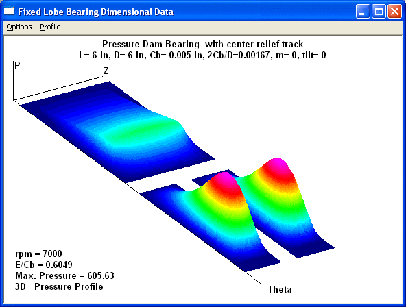
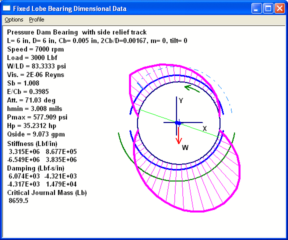
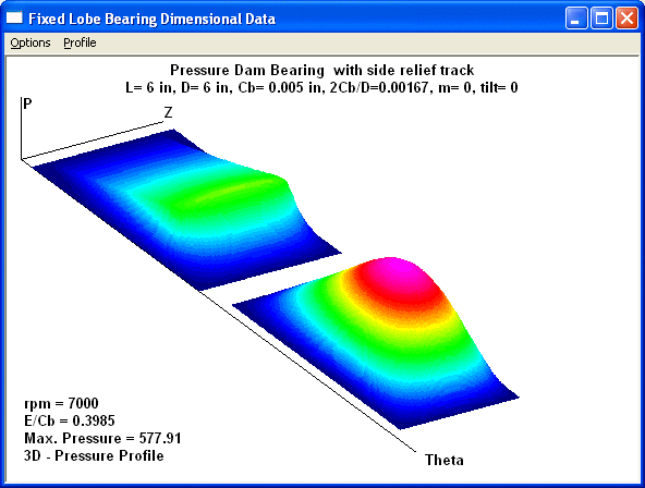
Note that, the central relief track can significantly lower the bearing load carrying capability. Therefore, caution must be taken when using the relief track. When the ReliefAxL is negative value, the relief track will be on both sides instead of at the center. The configuration with side relief track provides a better loading carrying capability than the central relief track. The same example with side relief track is illustrated below.
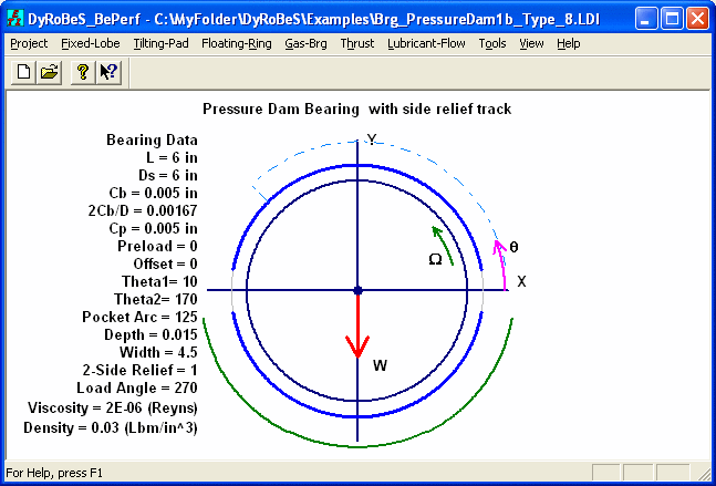
The bearing performance and pressure distribution are shown below.
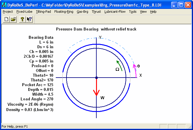
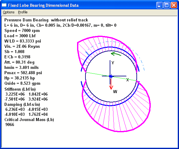
When ReliefAxL equals to zero, then no relief track is applied. The results are shown below.
Example 4: Tapered Land Bearing
A locomotive turbocharger bearing is employed in this example. It is machined out of a standard 3-axial groove bearing as shown in figures below. Again, the clearances, arc center offset, and undercut are exaggerated for illustration purposes. Each lobe is machined with an arc to form the tapered land. The arc has a radius of Ra and the arc center is specified with a center offset of r and an angle Theta measured from the reference axis (X-axis). The arc center angle normally is either in the middle of the oil groove or the same as the leading edge of the lobe. Typically, there are side dams in the tapered land area similar to the pressure dam bearing. When taper arc axial equals to the bearing axial length, no side dam exists. The circumferential taper arc length is normally not specified for a tapered land bearing since it will be the end of the arc. However, this arc length can be specified to form a step in the tapered land area.
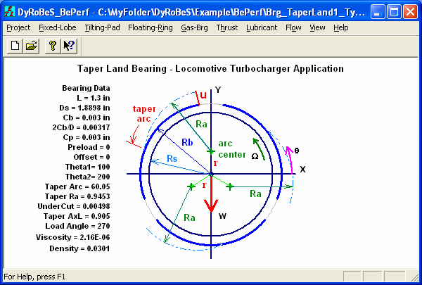
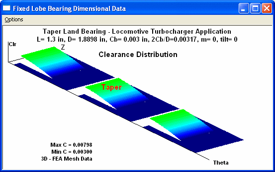
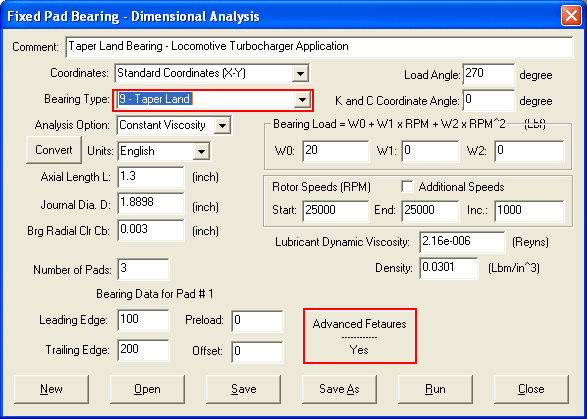
The input parameters for the tapered land bearing are shown below. Since the clearance is not continuous due to the side dams, Advanced Feature has to be ON. For the manufacturing drawing, the arc radius and arc center location (r, and theta) are normally specified. In the design process, the undercut and taper arc angle (length) are normally specified. For this purpose, a TOOLS button is provided in this dialog box. It allows the program users to specified any two parameters among the undercut (u), arc length (Arc theta), arc radius (Ra), and arc center offset (r) to calculate the other two unknowns.
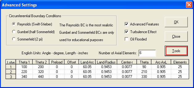
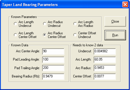
The results are present below.
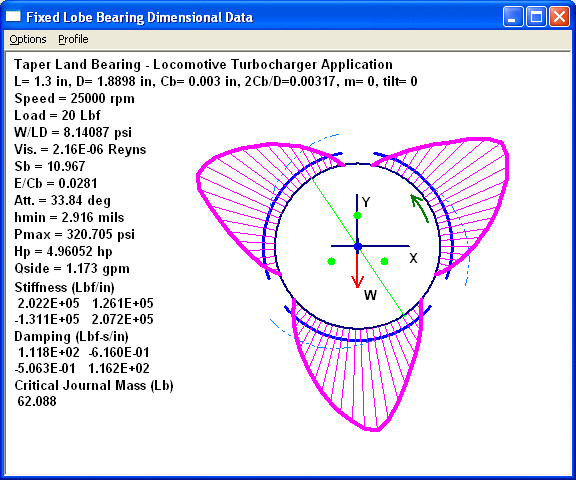
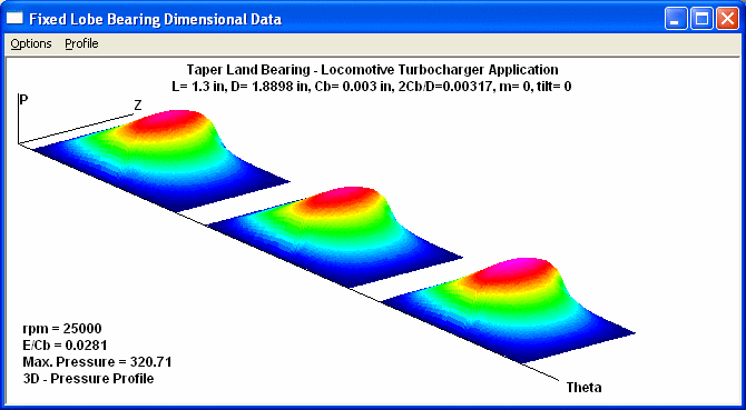
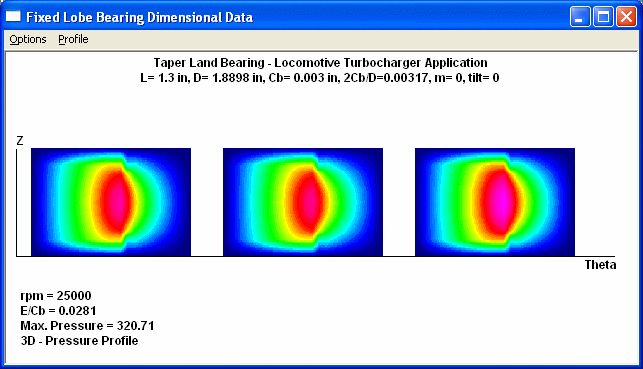
With this more general inputs, a pressure dam bearing without relief track can also be modeled with this bearing type.
Example 5: Step Bearing
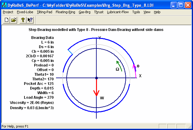
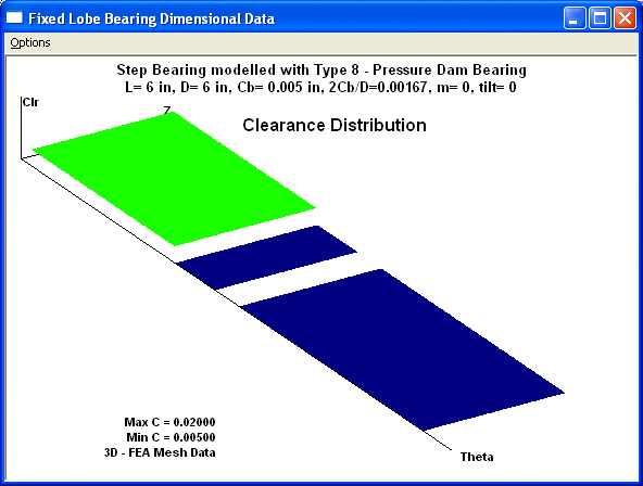
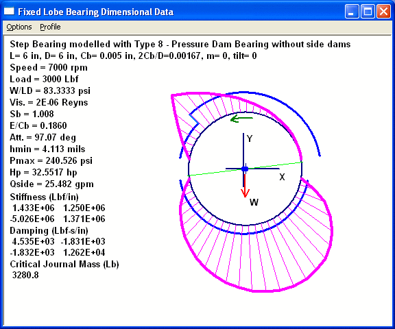
When the axial length of a pocket equals to the bearing axial length, it forms a step. A step bearing can be modeled using Type 8 – Pressure Dam Bearing with PocketAxL equals to the bearing axial length as demonstrated below.
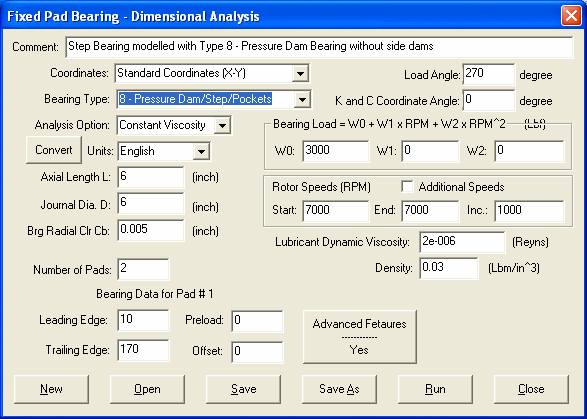
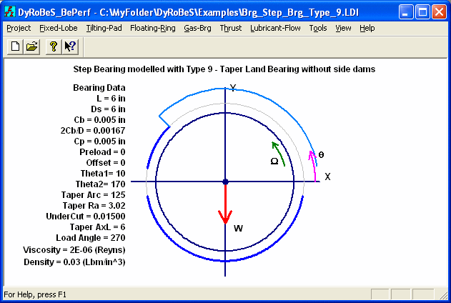
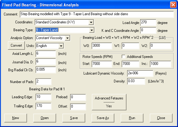
It can also be modeled with Type 9 – Taper Land Bearing as illustrated below. The results are identical in two cases.
Again, with the general inputs of pressure dam bearing and taper land bearing, more other types bearing can be modeled using these two types bearings.
Example 6: 5-Pads Tilting Pad Bearing
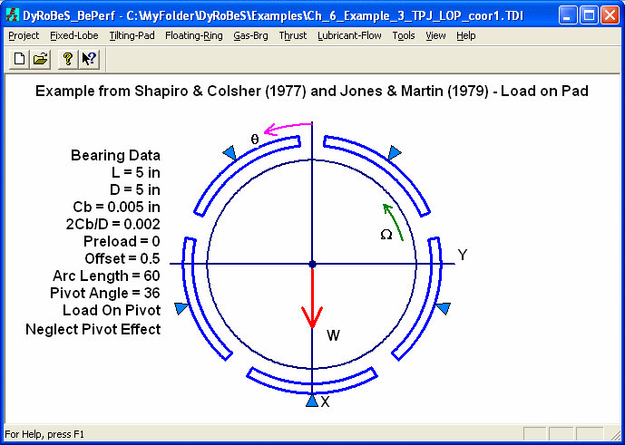
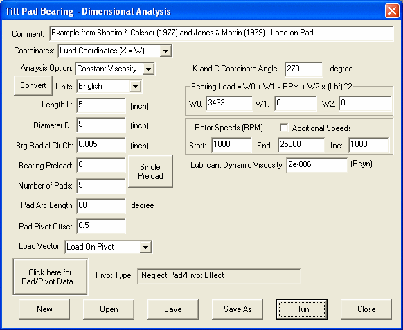
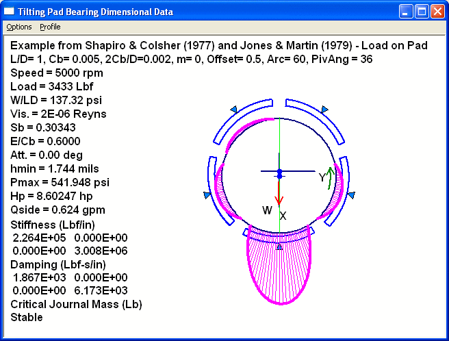
A 5-pads tilting pad bearing taken from Jones & Martin, ASLE Trans., 1979, is used in this example as shown below. For comparison purposes, Lund’s coordinate system is used, that is, the load vector is aligned with the X-axis. Lubricant viscosity is assumed to be constant and pivot/pad flexibility is ignored. The input parameters are shown for reference. The first case considered is Load On Pivot.
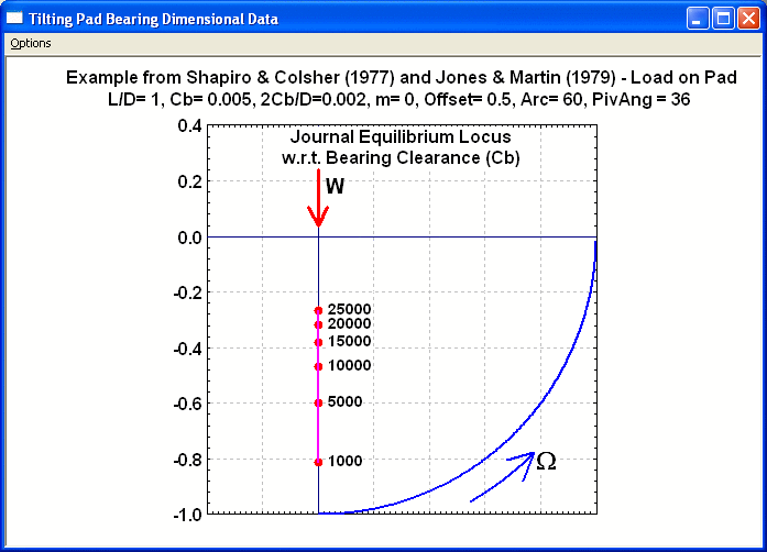
The results are presented below. Note that the bearing attitude angles are zero for the tilting pad bearings and the bearing cross-coupled stiffness coefficients are also zero. It indicates the inherently stable characteristics for the tilting pad bearings.
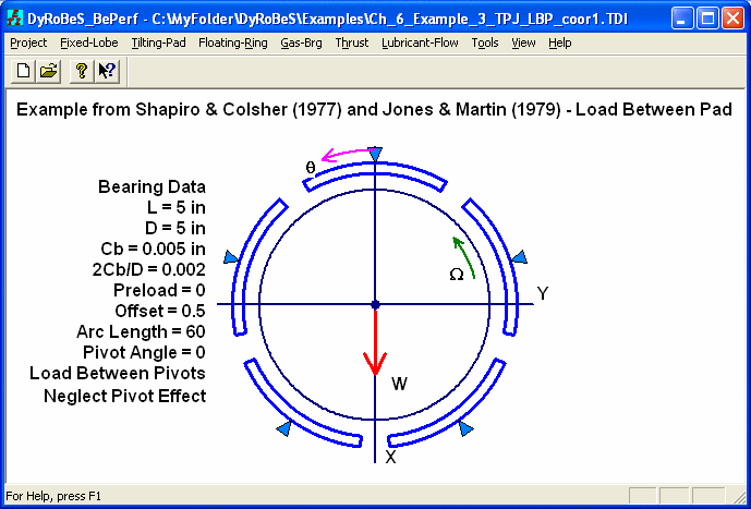
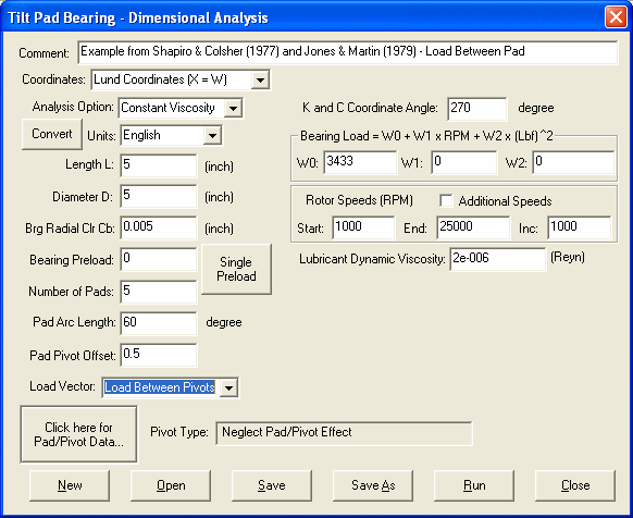
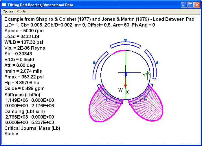
The second case considered is Load Between Pivots. The inputs and results are presented below.
Example 7: 4-Pads Tilting Pad Bearing – compressor application
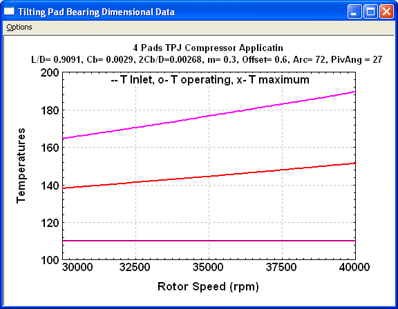
A 4-pads tilting pad bearing used in a gear driven centrifugal compressor is utilized in this example. The bearing load is mainly due to the gear force, which increases as the speed increases. For centrifugal compressor application, the gear load is a function of square of the rotor speed. Also, to lower the bearing maximum temperature, an pivot offset of 0.6 is used. The bearing is oriented such that the bearing load is directed between pivots. Note that the load vector is between pivots, not pads.
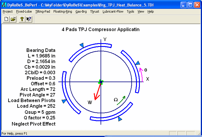
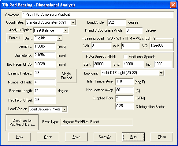
Some results are shown below:
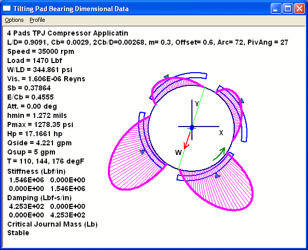
For 4-pads and load between pivots, the bearing stiffness and damping are identical in both X and Y directions. This implies that the bearing properties are isotropic.
Example 8: 4-Pads Tilting Pad Bearing with Pivot Flexibility
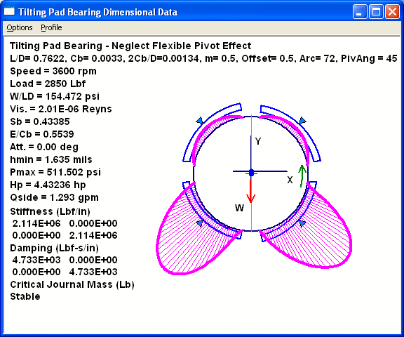
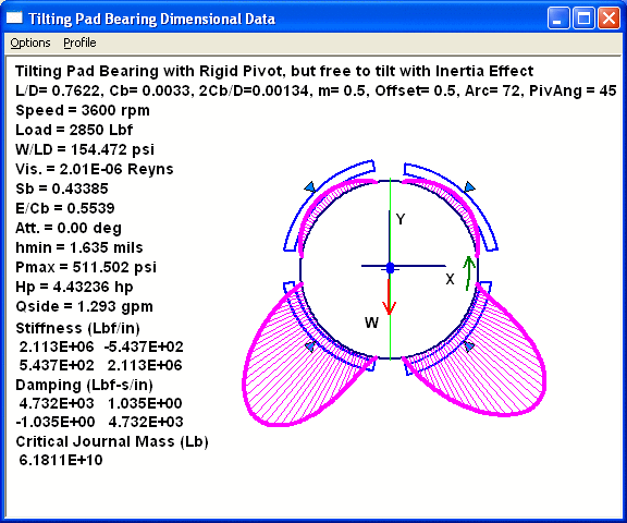
In this example, the pad/pivot flexibility is studied. For big bearings with larger pads, the pad effect may need to be included in the analysis. A tilting pad bearing used in the generator application is employed in this example. The bearing under study has spherical pivots. In this example, several different pad/pivot configurations are studied.
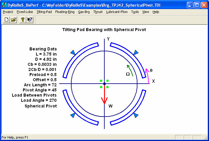
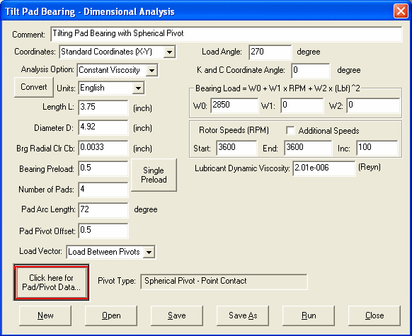
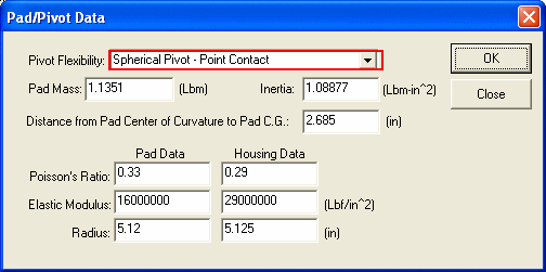
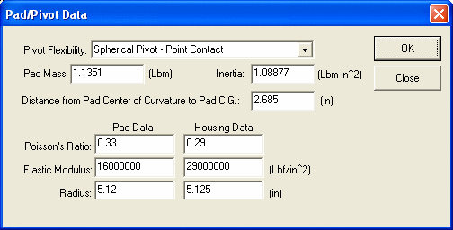
To select the pad/pivot configuration and enter the pad/pivot data, click the Pad/Pivot Data button as shown in the main input screen. They are several pivot configurations available in DyRoBeS.
Case 1 – Neglect Pad/Pivot Effect
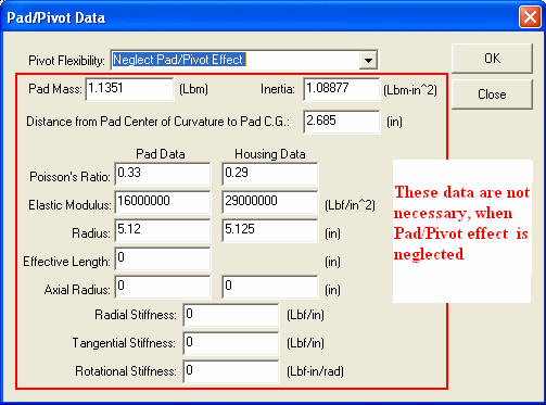
Case 2 – Rigid Pivot with inertia effect

Case 3 – Spherical Pivot, this is the true configuration.

Case 4 – General Curvatures, The spherical pivot can be modeled using this more general input.
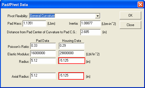

These results are identical to case 3. For Spherical Pivot and Cylindrical Pivot, the radii are always positive. For General Curvatures, the radii are positive if the center of curvature lies within the given body, i.e., the surface is convex, otherwise, the radii are negative.
Example 9: Floating Ring Bearing
Floating ring bearing is commonly used in the automotive turbocharger application. There are two oil films separated by a floating ring. It is like two bearings in series. For a conventional floating ring bearing, the ring is free to rotate. Then, two bearings are conventional plain cylindrical journal bearings. Sometimes, anti-rotational pin is used to prevent the ring from rotating, then, the outer oil film becomes a squeeze film damper. The bearing type of outer film, either plain journal bearing or squeeze film damper, depends on the speed ratio specified in the input. In this example, the ring is free to rotate.
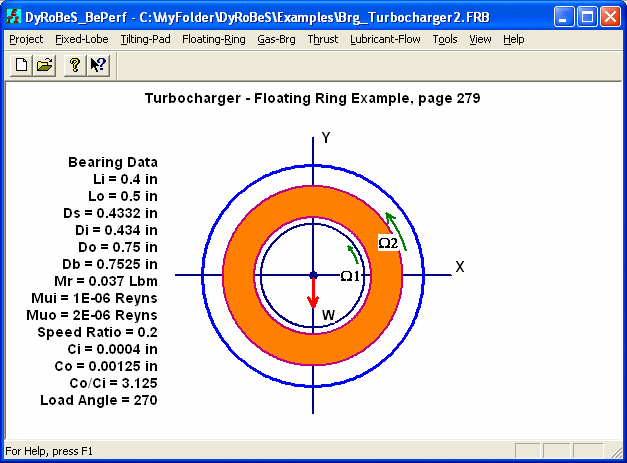
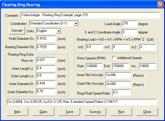
The temperature for the inner oil film is normally higher than that of the outer oil film, therefore, it has a smaller viscosity than that of outer film.
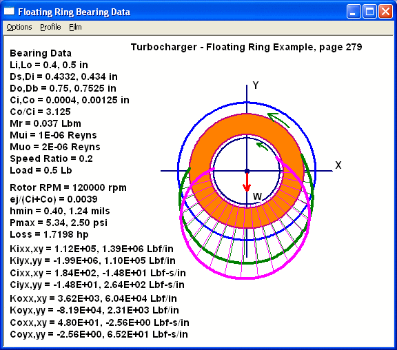
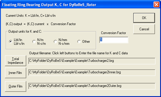
When outputs the bearing stiffness and damping coefficients, three files will be created. One is for the total impedance which synchronous excitation is assumed. The other two are the bearing stiffness and damping coefficients for the inner and outer films. It depends on how the rotor system is modeled. The users can make their decision on how to use these files.
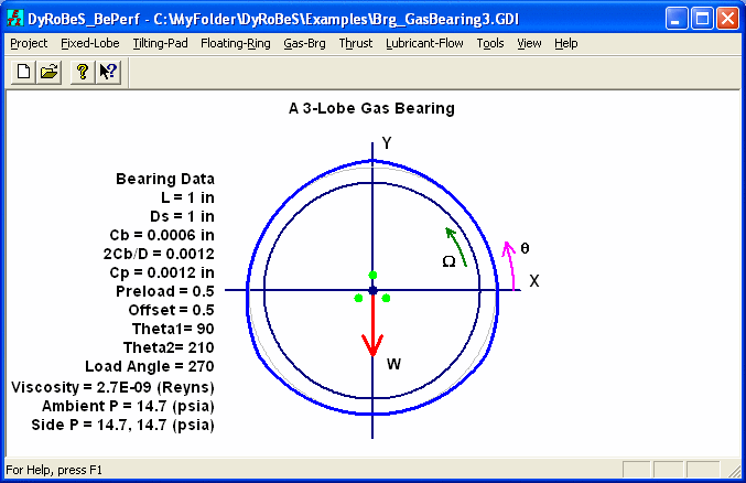
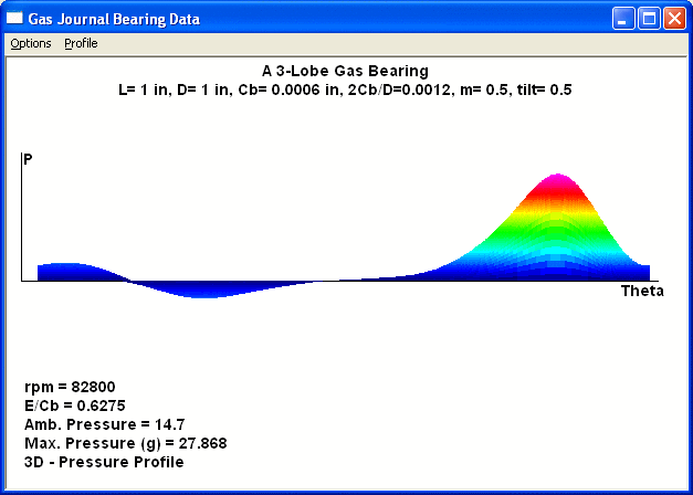
Example 10: A 3-Lobe Gas Bearing
A 3-lobe gas bearing is used in this example. The input parameters are shown below.
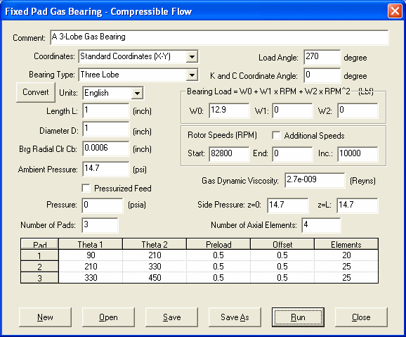
Some results are shown below.
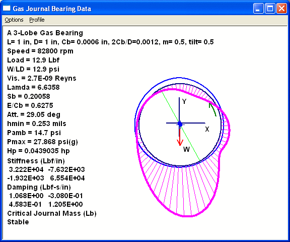
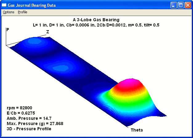
Copyright © 2014-2017