Whirl Speed and Stability Results
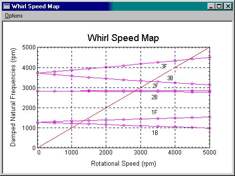
Whirl Speed Map is a linear plot of damped natural frequencies vs. shaft rotational speeds. The damped natural frequency is usually referred to as whirl speed. The damped critical speeds and any excitation resonance speeds are determined by noting the coincidence of the shaft speed with the system natural frequencies for a given excitation line in the Whirl Speed Map. A value of 1 in the excitation slope is associated with the synchronous excitation. Up to 5 excitation lines can be displayed in the plot by giving the different excitation slopes. The multiple excitation slopes are separated by commas. For example, the Excitation Slopes for the following display is set to be 1.0, 0.5. You can change the graph title, labels, number of modes, and many others by changing the default settings in the Setting dialog under Options menu.
Due to the non-symmetric properties of the bearing coefficients and the gyroscopic effect, the Whirl Speed Map can be very complicated, caution must be taken when preparing this map.
The following whirl speed map is generated for a typical rotor system with isotropic and constant bearing stiffness. At zero shaft speed, the forward and backward frequencies are identical (repeated eigenvalues). As the speed increases, each vibration mode is split into two modes known as forward and backward precessional modes due to the gyroscopic effect. For the forward precessional modes, the gyroscopic effect contributes negative kinetic energy and tends to raise the corresponding forward whirl frequency. For the backward precessional modes, the gyroscopic effect contributes positive kinetic energy and tends to lower the corresponding backward whirl frequency. Thus, it is the forward modes getting the gyroscopic stiffening effect and the backward modes getting the gyroscopic softening effect. The intersection between the synchronous excitation line and the damped natural frequencies are referred as damped critical speeds.
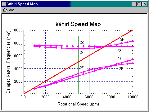
The following whirl speed map is generated for a rotor system supported by fluid film bearings. At the rotor speed of 5000 rpm, the first mode is a forward conical mode and the second mode is a forward translational mode. The first two backward modes are overdamped (real modes) in this example and are not shown in this map. The third mode is a forward bending mode and the fourth mode is a backward bending mode. However, at the rotor speed of 10000 rpm, the first mode becomes a forward translational mode and the second mode becomes conical mode. The third mode now is a backward bending mode and the fourth mode is a forward bending mode. The direction of precession (forward or backward) and the type of modes (rigid body, bending) should be determined from the mode shapes not from the whirl speed map.
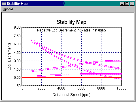
Stability Map
Stability Map is a linear plot of logarithmic decrements (or damping factors) vs. shaft rotational speeds. Negative logarithmic decrement indicates system instability. When the value of logarithmic decrement exceeds 1, that particular mode is well damped. As shown in the figure, the logarithmic decrement of the first mode approaches to zero as the rotor speed approaches to 9100 rpm, and then becomes negative as the rotor speed increases. This speed is known as the instability threshold. Self-excited instability occurs at the speeds above the instability threshold.
You can change the graph title, labels, number of modes, and many others by changing the default settings in the Setting dialog under Options menu.
Due to the non-symmetric properties of the bearing coefficients and the gyroscopic effect, the Stability Map can also be very complicated, caution must be taken when preparing this map.
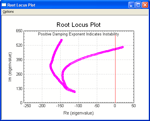
Root Locus Plot
Root locus plot is also commonly used in the system stability evaluation, particularly by control engineers. It is a plot with imaginary part of eigenvalue vs. the real part of eigenvalue for a range of rotor speed as shown below. In DyRoBeS, the imaginary part can also be the cycle per minute or Hz and the real part can be the logarithmic decrement or damping factor.
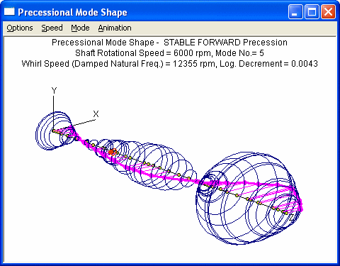
3D Precessional Mode Shapes
This plot displays a three-dimensional precessional mode shape. The 3-D mode shapes can be displayed in different views by adjusting the Display Projection option in the Settings. You can quickly switch the speed and mode number by using the Speed and Mode options. You can change many other features by changing the default settings in the Setting dialog under Options menu. Animation option allows you to animate the motion and it is easy to see the forward, backward, or mixed precession.
See also Lateral Vibration Analysis, Whirl Speed and Stability Analysis.
Copyright © 2014-2017